Oil Demand Through The Energy Transition
Summary
This paper was written in November 2020 following the publication of updated long term oil demand forecasts by the International Energy Agency (IEA), The US Energy Information Administration (EIA), the Organisation of the Petroleum Exporting Countries (OPEC) and bp. The objective of the paper is to compare and evaluate the various forecasts, apply a quantitative framework to determine which path is the most likely and explore the implications of that path for the E&P industry.
The first section of the paper compares the demand forecasts, providing some qualitative commentary on the validity of each. This section concludes that the forecasts are broadly divided into those that predict continuing oil demand growth and those that predict dramatic oil demand decline, and they are divergent, predicting oil demand at anywhere between 25 MMbbl/day and 130 MMbbl/day by 2050.
The second section of the paper looks at William Nordhaus’s work on carbon pricing and uses some of his insights to assess the oil demand forecasts more quantitatively. The conclusion from this section is that another one to two decades of oil demand growth is the most likely outcome, as decarbonizing the power sector is the most cost effective and politically feasible area for carbon dioxide abatement in the first instance.
The third section of the paper explores the impact of this scenario on the E&P industry, in terms of market dynamics, when oil demand does begin to fall. This section concludes that investment in new field development will taper down rapidly when demand begins to decline, resulting in a period of high oil prices. Low operating costs for existing fields will be of greater importance for E&P companies than low lifecycle breakeven prices and in this environment US shale will emerge as the asset of choice, given its short cycle times and rapid payback.
Long Term Oil Demand Forecast
All the major institutions that provide long term demand forecasts for oil have now published their 2020 updates. These are the IEA (i) , the EIA (ii), OPEC (iii) and bp (iv). All of these, with the exception of the EIA, have been updated to incorporate the impact of COVID-19. While the EIA have published an update, they have not updated their base demand forecast, as they only do this in alternate years.
Consequently, the EIA forecast has been rebaselined to allow for comparison. The approach taken was to assume the latest IEA demand estimates for 2020 and 2021, then assume a return to 2019 demand levels, 99.8 MMbbl per day, in 2022. As the IEA still assumes significant COVID-19 impact to air travel in 2021, the assumption of some remaining demand rebound potential into 2022 seems valid. Having set a new baseline in 2022, the annual percentage demand increase or decrease from the reference year in the original forecast was applied. The demand forecasts are shown in Figure 1, below. This shows a range of projected oil demand, by 2050, of between 25 MMbbl/day and 130 MMbbl/day.
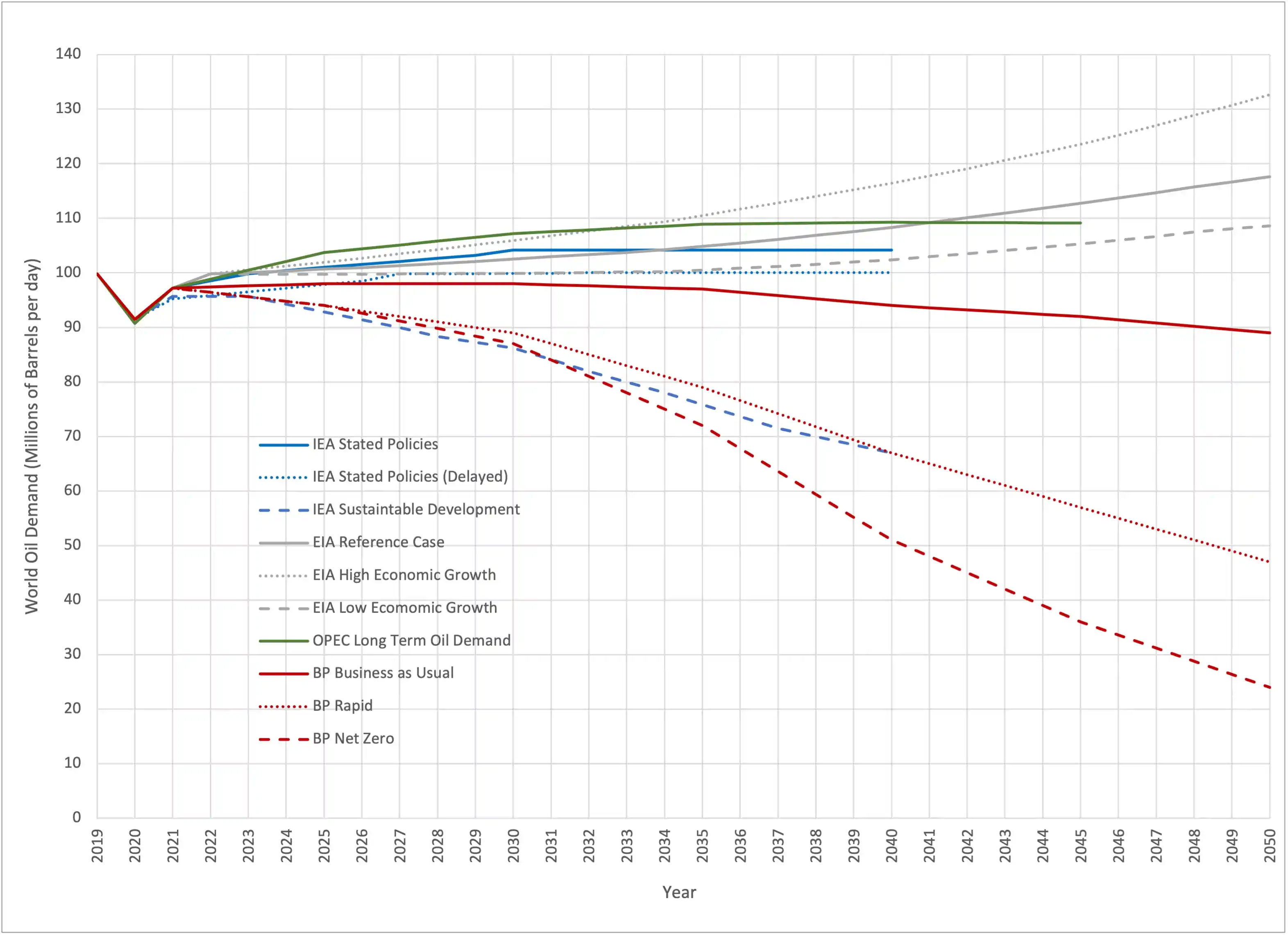
Figure 1 - Comparison of Long-Term Oil Demand Forecasts
The first challenge in evaluating these forecasts is that the underlying assumptions that drive the forecast and the future that each envisages are not explained, consequently there is a fair amount of inference in each case. The second challenge is that each of the forecasts provide demand at a given point in time – 2030, 2035 and so on – but not the years in between and so some interpolation is required. This makes medium term forecasting – from 2020 to 2025 for example, quite difficult.
If we start with the EIA, it has the highest long-term oil demand forecasts. They appear to be tied to projections of long-term economic growth, with demand growth accelerating towards the middle of the century. There has been a historic correlation between economic growth and oil demand but projecting that relationship into the future fails to acknowledge that emergent technologies like electric vehicles and videoconferencing and changes in societal attitudes to things like recycling will weaken that relationship. Consequently, the EIA forecasts have been discounted as they tend to overestimate the potential for demand growth.
In the IEA stated policies case, demand recovers to 2019 levels in 2023 and peak demand is shifted down from 106 MMbbl per day to about 104 MMbbl per day in 2030. The IEA had added a stated policy delayed recovery case, where demand reaches 2019 levels in 2027 and flatlines at that level through 2040. Neither IEA forecasts predict demand decline, except for 2020, through the forecast period. The IEA has also adjusted their sustainable policies forecast, which now shows a much steeper dip in demand over the next decade, before reverting to its 2019 path.
OPEC have extended their forecast period from 2040 to 2045 and cut about 1.3 MMbbl/day from their peak demand estimate; this is now 109.2 MMbbl per day in 2040. OPEC sees demand recovering to 2019 levels in 2022, a year ahead of the IEA. OPEC predicts 2040 will be the peak demand year, with demand declining slowly to 109.1 MMbbl per day in 2045.
One of the most difficult forecasts to form a view on is bp’s ‘Business as Usual’ case because it is difficult to understand what it is based on. Where details of underlying assumptions were provided, some of them a looked questionable. The figure below is taken from one of bp’s Energy Outlook slides and shows the projected adoption of Robotaxi’s measured in vehicle kilometer miles (VKM) traveled. bp’s ‘Business as Usual’ scenario shows this jumping from essentially 0% to 20% of all vehicle miles traveled over a 5-year period, which given the technology doesn’t currently exist and the US vehicle fleet turns over every 10 – 15 years, doesn’t seem very credible. For some reason ‘Business as Usual’ yields a higher Robotaxi penetration than the more aggressive transition scenarios, which doesn’t seem internally consistent, and then penetration drops off in all scenarios, which again doesn’t make sense if Robotaxis are the way of the future.
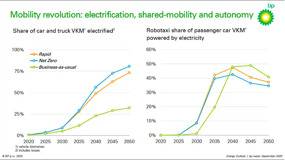
Figure 2 - Robotaxi Slide from bp Energy Outlook presentation
Spencer Dale, to his credit, introduced bp’s new demand forecasts by pointing out they would all be wrong and that the purpose of these scenarios is to explore the full range of possible futures. He then went on to say that all the scenarios were premised on a sustained decline in an existing energy source, something that has never happened in the history of traded fuels, and transition to new energy sources at an unprecedented rate. This is 2020, we have all been recently reminded that unprecedented things happen, but to premise all your scenarios on two unprecedented things happening suggests that the scenarios are too narrowly drawn. At least one of them should conform to historical norms, to test what that future would look like. Given this, the IEA ‘Stated Policies’ and the OPEC forecast seem more credible.
Of the lower scenarios, bp’s ‘Rapid’ and ‘Net Zero’ cases and the IEA’s ‘Sustainable Development’ case stand out. All of these see oil demand falling by 10 MMbbl/day over the next decade and accelerating at different rates from there. bp’s ‘Rapid’ and ‘Net Zero’ cases conform to the carbon budget required to limit global warming to less than 2 degrees centigrade and 1.5 degrees centigrade respectively. The basis of the IEA’s ‘Sustainable Development’ scenario, which is very similar to the BP ‘Rapid’ scenario, is based on exactly that premise. These then can be seen not so much as forecasts of what will happen, but as illustrations of what would have to happen, to meet a certain carbon budget.
A recent publication by McKinsey (v) examined what would be required to accelerate peak oil demand to the mid 2020’s. The dominant factor was accelerated electrical vehicle penetration, with reduced plastic demand and an increase in recycling also playing a role. This would see oil demand fall to 80 MMbbl/day by 2035, in line with IEA ‘Sustainable Development’ scenario or bp’s ‘Rapid’ scenario. To realize this future, annual electric vehicle demand as a proportion of total car sales, would need to rise from less than 1% in 2018, to nearly 6% in 2020, to more than 30% by 2025. While this outcome may not be the most likely, it doesn’t seem to be impossible as sales in 2019 reached 2.6% of the total, and so the IEA ‘Sustainable Development’ or bp ‘Rapid’ scenario could be a lower bound to demand.
The range of forecasts for oil demand in 2050 remains between 25 MMbbl/day and 130 MMbbl/day. The forecasts also bifurcate, with half ‘above the line’ in that they predict modest demand growth through the next decade or so, and the other half ‘below the line’ in that they predict an aggressive decline in oil demand from 2019 levels. The next section of this report looks at some of the work that has been done on carbon pricing, to allow the forecasts to be assessed under a more quantitative framework, in order to understand why they are so different and which outcomes are more likely.
The Social Cost of Carbon
William Nordhaus, a Yale professor, who won the Nobel prize in economics in 2018 for his work on climate change, developed a model that quantified the impact of carbon emissions on the world economy. The model is used to calculate the cost to society of carbon emissions in terms of abatement, the cost of reducing carbon emissions, and damages, the cost imposed on society by climate change.
He used this model to estimate the cost of inaction on climate change as well as imposing various climate change policies, expressed as a social cost of carbon, the cost to society of emitting carbon dioxide (vi). He also used the model to calculate an optimized economic path, mixing abatement and damage, that minimized the costs to society of carbon dioxide emissions. He advocates a global carbon tax to reduce carbon dioxide emissions, with his model providing a guide to the level at which the tax should be set, to achieve a given level of warming.
Current climate policies are a patchwork, with some countries such as Sweden, applying an effective carbon tax as high as $127 per ton of carbon dioxide on some sectors of their economy, while 80% of emissions globally are not taxed at all. The result is that the world currently taxes carbon dioxide emissions at an effective rate of $1.70 per ton (vii). In the NBER paper, William Nordhaus looked at a base case, an optimal case, a 2.5 degree centigrade limit case and the Stern case, which uses a very low discount rate. The two charts below are reproduced from his paper and show annual carbon dioxide emissions reductions and the associated temperature increase.

Figure 3 - Global CO2 Emissions from NBER Paper
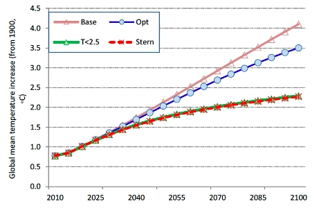
Figure 4 - Temperature Change from NBER Paper
There is no 1.5 degree or 2.0 degree limit case in the paper and looking at the reduction in carbon dioxide emissions required for a 2.5 degree limit, those targets do indeed look practically impossible. In the base case, Figure 4 shows the world would be more than 4 degrees centigrade warmer in 2100 and in the optimal case, it would be about 3.5 degrees warmer. Referring to Figure 3, there is a very substantial decrease in carbon dioxide emissions required to achieve that relatively small difference in outcome.
Figure 5 shows the cost to society of carbon dioxide emissions under the various scenarios using data from the NBER report. Table 1 shows the cost of carbon dioxide emissions on an annualized basis using data taken from the NBER report. There are two conclusions from Figure 5. The first is that the optimal path imposes the lowest costs on society. The second is that the base case imposes significantly lower costs than trying to limit global warming to 2.5 degrees centigrade in 2100.
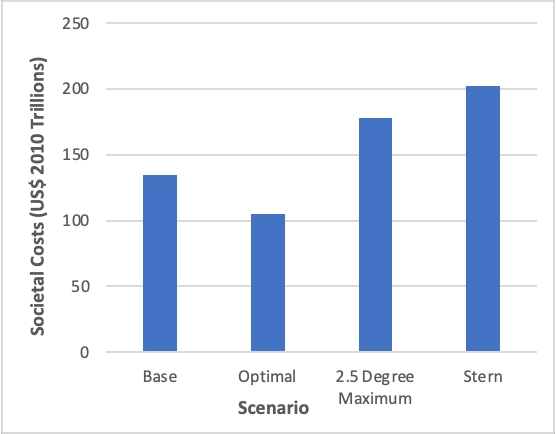
Figure 5 - Societal Cost of Climate Change
From Table 1, we can see that there is no real difference in the annual cost of carbon between base and optimum scenarios. The difference between the two is that there is less damage under the optimal case and more abatement. The real benefits of the optimal case are realized in the second half of the century.

Table 1 - Social Cost of Carbon Annually ($ / Ton)
There are some legitimate criticisms of this approach. After all, none of us live in an economic model, but in a world that will be noticeably warmer. Like all models it is, at best, directionally correct and over long time horizons economics discounts away damage in the distant future. It does, however, provide a tool to estimate the costs and benefits of action, which is a lot better than no tool at all.
What would be the impact of imposing a carbon tax of $50 or $100 per ton on oil demand? Columbia’s Center for Global Energy Policy have looked at the impact for energy demand in the United States based on carbon taxes of between $0 and $73 per ton (viii). Their conclusion was that a tax would result in a substantial reduction in carbon dioxide emissions but would have almost no impact on oil demand. This is because a carbon tax works by eliminating the cheapest emissions first; the Colombia paper found that almost all the reduction in emissions came in the power sector, where renewables and natural gas replaced coal, because those replacement fuels are already economically competitive. A carbon tax of $50 per ton would equate to a $0.44 dollar per gallon tax on gasoline. This is about 20% of the cost of the average 2016 tank of gasoline, which was $2.30, an increase which falls well within the range of fluctuations in gasoline prices driven by the oil price. Table 2 shows the impact on a gallon of gasoline for the carbon taxes shown in Table 1.

Table 2 - Additional Tax on Gasoline ($/Gallon)
The Colombia study did not examine the impact of the $2 plus taxes on carbon emissions, but it isn’t hard to imagine that doubling, tripling and then quadrupling the cost of gasoline would have a dramatic impact on demand.
Bringing the discussion back to long term oil demand forecasts, this divergence in carbon rates under different scenarios can explain the divergence in forecasts. The ‘above the line’ forecasts, those that predict demand rising for the next decade or two, follow a base or optimized carbon price path, where abatement of carbon dioxide emissions will be focused on the power sector. The ‘below the line’ forecasts follow a temperature limited path, where the abatement impact of the mobility sector are dramatic and immediate.
It seems unlikely that society would be willing to accept, or that politicians could be reelected after imposing, the kinds of costs that would be required to achieve the ‘below the line’ forecasts. It is hard to imagine the US government attempting to impose a $2 per gallon gasoline tax and increasing it at 10 cents per year. The aggressive bp forecasts and the IEA sustainable development case would restrict temperature rise to 1.5 degree or below 2.0 centigrade, implying even higher gasoline taxes than that. The ‘above the line’ forecasts reflect not only the economic optimum, but also the political reality, which means that oil demand can be expected to continue to grow for the next ten to twenty years.
Implications for the E&P Industry
If we adopt this oil demand scenario, what are the implications for the E&P industry? Some media coverage earlier this year suggested that the COVID-19 pandemic foreshadowed what this decline in demand would look like for the industry. As a reminder, if any were needed, April this year saw oil demand collapse by 12.4 MMbbl/day month on month at the same time as Saudi Arabia initiated a price war by adding 2 MMbbl/day to global supply. This doesn’t seem a suitable analogue for structural demand decline, which is likely to be gradual and sustained over decades. It is likely that peak demand won’t be recognized until several years after the event, and post plateau underlying demand decline rates of 1%-2%, of a similar magnitude to pre-plateau demand growth rates, seem more likely.
What are the implications for the industry under this scenario? The major international oil companies have consistently pointed out that the world will need oil, and new supplies of oil, for decades to come, which is consistent with the scenario outlined here. The emphasis has been on developing assets with low breakeven prices, so that when demand declines, those assets will remain competitive while assets with higher break evens will have their production pushed out of the market. This strategy makes intuitive sense. Does that mean that business will continue as normal?
Figure 6, below, is taken from a recent press release by Rystad Energy (ix). This figure shows the breakeven price of oil supply, broken out by theme. Breakeven prices are on a point forward basis and it appears that averages are used rather than actual field data, as the legend indicates a 60% confidence interval around the average breakeven price presented.
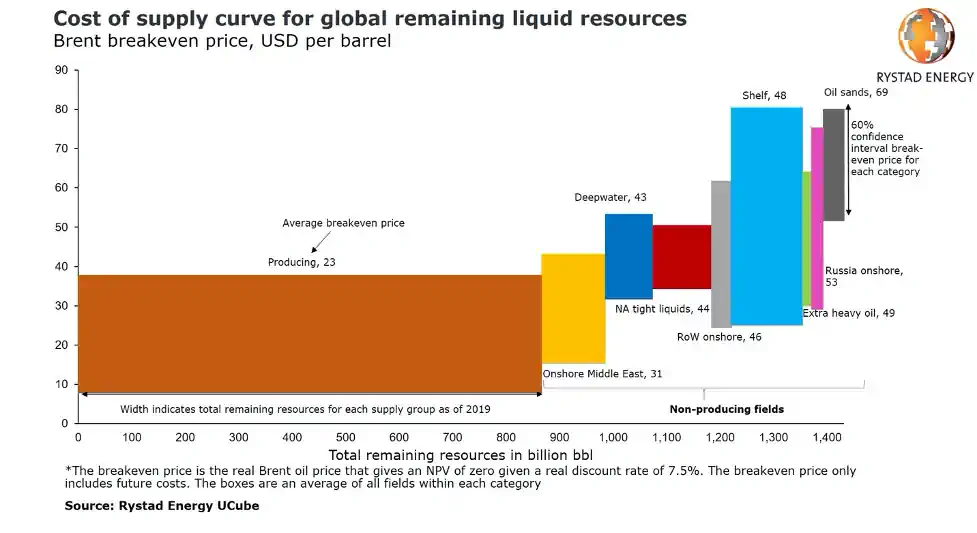
Figure 6 - Oil Supply Cost Curve
Figure 6 distinguishes between producing and non-producing fields and the key takeaway from this chart is that, using average costs on a point forward basis, there is no field development theme that can compete with existing production. Figure 6 is a simplification, within each theme there will obviously be a range of breakeven prices, which will change for each field over time as production declines with age. There will also be fields, in the middle east and perhaps deep water fields in places such as Guyana and Brazil, that can compete with existing production, even including their capital cost. Notwithstanding these points, broadly speaking non-producing fields will struggle to compete with producing fields on breakeven price. This conclusion makes intuitive sense, after all, non-producing fields still require capital investment to bring them on stream, whereas for producing fields, that is a sunk cost. This implies that new production from non-producing fields will not displace existing production from producing fields.
The second point of difference between existing production and non-producing fields is how operational and investment decisions are made. In a producing field, the decision on whether to continue or suspend production is made on the basis of whether the field can be operated profitably, together with a consideration of the value of deferring abandonment. Oil price risk can be transferred by hedging production over the next year or 18 months. Decisions are made over a short time horizon with high certainty. Compare this to a non-producing field. Even those fields that are ready to take a Final Investments Decision are years away from realizing first production, with the return on investment then being made over a further 15 to 30 year period. There is no way to transfer price risk by hedging. In contrast to existing production, decisions are taken over very long time horizons with high uncertainty. The investment case has worked historically because oil demand was rising. How can a company justify the risk associated with that kind of long term investment when demand declines?
The implication of this second point is that investment in new oil fields will cease once demand begins to decline. It won’t, of course, stop everywhere at once, but it will taper down with the only the most profitable, short cycle fields continuing to attract investment, until eventually even those are considered to be too high risk.
What does this type of scenario mean for the industry today? In the first instance, the role of exploration in the oil and gas industry will change; it will shrink and shift in focus to infrastructure led opportunities that can be quickly monetized. BP has already announced that it is moving down this route, by abandoning exploration in new basins. Their timing may turn out to be prescient but given the assumption of another decade or two of demand growth, it seems a little early. There are still a lot of high value exploration opportunities available and enough time to monetize them.
This scenario also calls into question the industries current strategy of focusing on fields with low breakeven prices, at least for the next decade or so. Of course, low breakeven prices are always important to the extent that they are also a reflection of overall field profitability, but providing the field is sanctioned within the next decade or two, that production will not be displaced. Under this scenario, low operating costs will be more important over the long run than low lifecycle breakeven prices.
What does the future oil market look like under this kind of scenario? It is intuitive to think that a world in which oil demand declines would be characterized by consistently low prices. But a world in which demand declines at 1%-2% while underlying production declines at 5% and there is no material new investment, is a world in which oil prices would soar. This would be a world in which field redevelopment and infill drilling opportunities could become highly profitable, but they are unlikely to be enough to fill the void.
The kind of asset that would really win in this environment would be one that has no exploration risk, could be brought on stream in months rather than years and which realizes the bulk of its economic value over a time horizon where price risk can be transferred through hedging. If this description sounds familiar, it should. US shale is the ideal asset for a world where oil demand is declining as it has exactly those characteristics. It may turn out that the US shale revolution of the last decade was just a couple of decades early.
To summarize, the scenario presented here is one in which oil demand continues to rise for the next decade or two, plateauing and beginning a slow and steady decline. Once this occurs, investment in new oil and gas fields will quickly decline, resulting in price spikes as underlying field production declines outstrip the decline in supply. US shale becomes the asset of choice, given its short cycle times and the ability to realize most of the value within 18 months of investment.
The best strategy for an oil and gas company to pursue under this scenario is to invest in long life assets with low operating costs, not necessarily the assets with the lowest lifecycle breakeven prices. Maintain an active exploration program, including new basin exploration, and only begin to exit these positions when the projected first oil dates from these fields moves beyond 2035 – 2040. Take advantage of the currently depressed US shale industry to assemble a competitive shale position; a position that can be held over the long term with minimum work commitments. While this is an oil focused article, continuing to invest in profitable gas and renewable opportunities should also form part of this strategy.
(i) IEA (2020), World Energy Outlook 2020, IEA, Paris https://www.iea.org/reports/world-energy-outlook-2020
(ii) “International Energy Outlook 2020”, Energy Information Administration, October 2020
(iii) World Oil Outlook 2045, October 2020, OPEC
(iv) Energy Outlook 2020 Edition, September 2020, bp
(v) Global Energy Perspective: Accelerated Transition, November 2018, Energy Insights by McKinsey
(vi) “Projections and Uncertainties about climate change in an era of minimal climate policies”, National Bureau of Economic Research Working Paper 22933, William D. Nordhaus, September 2017.
(vii) “Climate Change: Our Ultimate Challenge”, William Nordhaus, Lecture at the University of Zurich, January 21st, 2020.
(viii) “Energy and Environmental Implications of a Carbon Tax in the United States”, Columbia Center on Global Energy Policy, July 2018.
(vix) “Oil production costs reach new lows, making deep water one of the cheapest sources of novel supply”, Rystad Energy, October 21st, 2020.
Conversation


Oil Demand Through The Energy Transition
Summary
This paper was written in November 2020 following the publication of updated long term oil demand forecasts by the International Energy Agency (IEA), The US Energy Information Administration (EIA), the Organisation of the Petroleum Exporting Countries (OPEC) and bp. The objective of the paper is to compare and evaluate the various forecasts, apply a quantitative framework to determine which path is the most likely and explore the implications of that path for the E&P industry.
The first section of the paper compares the demand forecasts, providing some qualitative commentary on the validity of each. This section concludes that the forecasts are broadly divided into those that predict continuing oil demand growth and those that predict dramatic oil demand decline, and they are divergent, predicting oil demand at anywhere between 25 MMbbl/day and 130 MMbbl/day by 2050.
The second section of the paper looks at William Nordhaus’s work on carbon pricing and uses some of his insights to assess the oil demand forecasts more quantitatively. The conclusion from this section is that another one to two decades of oil demand growth is the most likely outcome, as decarbonizing the power sector is the most cost effective and politically feasible area for carbon dioxide abatement in the first instance.
The third section of the paper explores the impact of this scenario on the E&P industry, in terms of market dynamics, when oil demand does begin to fall. This section concludes that investment in new field development will taper down rapidly when demand begins to decline, resulting in a period of high oil prices. Low operating costs for existing fields will be of greater importance for E&P companies than low lifecycle breakeven prices and in this environment US shale will emerge as the asset of choice, given its short cycle times and rapid payback.
Long Term Oil Demand Forecast
All the major institutions that provide long term demand forecasts for oil have now published their 2020 updates. These are the IEA (i) , the EIA (ii), OPEC (iii) and bp (iv). All of these, with the exception of the EIA, have been updated to incorporate the impact of COVID-19. While the EIA have published an update, they have not updated their base demand forecast, as they only do this in alternate years.
Consequently, the EIA forecast has been rebaselined to allow for comparison. The approach taken was to assume the latest IEA demand estimates for 2020 and 2021, then assume a return to 2019 demand levels, 99.8 MMbbl per day, in 2022. As the IEA still assumes significant COVID-19 impact to air travel in 2021, the assumption of some remaining demand rebound potential into 2022 seems valid. Having set a new baseline in 2022, the annual percentage demand increase or decrease from the reference year in the original forecast was applied. The demand forecasts are shown in Figure 1, below. This shows a range of projected oil demand, by 2050, of between 25 MMbbl/day and 130 MMbbl/day.

Figure 1 - Comparison of Long-Term Oil Demand Forecasts
The first challenge in evaluating these forecasts is that the underlying assumptions that drive the forecast and the future that each envisages are not explained, consequently there is a fair amount of inference in each case. The second challenge is that each of the forecasts provide demand at a given point in time – 2030, 2035 and so on – but not the years in between and so some interpolation is required. This makes medium term forecasting – from 2020 to 2025 for example, quite difficult.
If we start with the EIA, it has the highest long-term oil demand forecasts. They appear to be tied to projections of long-term economic growth, with demand growth accelerating towards the middle of the century. There has been a historic correlation between economic growth and oil demand but projecting that relationship into the future fails to acknowledge that emergent technologies like electric vehicles and videoconferencing and changes in societal attitudes to things like recycling will weaken that relationship. Consequently, the EIA forecasts have been discounted as they tend to overestimate the potential for demand growth.
In the IEA stated policies case, demand recovers to 2019 levels in 2023 and peak demand is shifted down from 106 MMbbl per day to about 104 MMbbl per day in 2030. The IEA had added a stated policy delayed recovery case, where demand reaches 2019 levels in 2027 and flatlines at that level through 2040. Neither IEA forecasts predict demand decline, except for 2020, through the forecast period. The IEA has also adjusted their sustainable policies forecast, which now shows a much steeper dip in demand over the next decade, before reverting to its 2019 path.
OPEC have extended their forecast period from 2040 to 2045 and cut about 1.3 MMbbl/day from their peak demand estimate; this is now 109.2 MMbbl per day in 2040. OPEC sees demand recovering to 2019 levels in 2022, a year ahead of the IEA. OPEC predicts 2040 will be the peak demand year, with demand declining slowly to 109.1 MMbbl per day in 2045.
One of the most difficult forecasts to form a view on is bp’s ‘Business as Usual’ case because it is difficult to understand what it is based on. Where details of underlying assumptions were provided, some of them a looked questionable. The figure below is taken from one of bp’s Energy Outlook slides and shows the projected adoption of Robotaxi’s measured in vehicle kilometer miles (VKM) traveled. bp’s ‘Business as Usual’ scenario shows this jumping from essentially 0% to 20% of all vehicle miles traveled over a 5-year period, which given the technology doesn’t currently exist and the US vehicle fleet turns over every 10 – 15 years, doesn’t seem very credible. For some reason ‘Business as Usual’ yields a higher Robotaxi penetration than the more aggressive transition scenarios, which doesn’t seem internally consistent, and then penetration drops off in all scenarios, which again doesn’t make sense if Robotaxis are the way of the future.

Figure 2 - Robotaxi Slide from bp Energy Outlook presentation
Spencer Dale, to his credit, introduced bp’s new demand forecasts by pointing out they would all be wrong and that the purpose of these scenarios is to explore the full range of possible futures. He then went on to say that all the scenarios were premised on a sustained decline in an existing energy source, something that has never happened in the history of traded fuels, and transition to new energy sources at an unprecedented rate. This is 2020, we have all been recently reminded that unprecedented things happen, but to premise all your scenarios on two unprecedented things happening suggests that the scenarios are too narrowly drawn. At least one of them should conform to historical norms, to test what that future would look like. Given this, the IEA ‘Stated Policies’ and the OPEC forecast seem more credible.
Of the lower scenarios, bp’s ‘Rapid’ and ‘Net Zero’ cases and the IEA’s ‘Sustainable Development’ case stand out. All of these see oil demand falling by 10 MMbbl/day over the next decade and accelerating at different rates from there. bp’s ‘Rapid’ and ‘Net Zero’ cases conform to the carbon budget required to limit global warming to less than 2 degrees centigrade and 1.5 degrees centigrade respectively. The basis of the IEA’s ‘Sustainable Development’ scenario, which is very similar to the BP ‘Rapid’ scenario, is based on exactly that premise. These then can be seen not so much as forecasts of what will happen, but as illustrations of what would have to happen, to meet a certain carbon budget.
A recent publication by McKinsey (v) examined what would be required to accelerate peak oil demand to the mid 2020’s. The dominant factor was accelerated electrical vehicle penetration, with reduced plastic demand and an increase in recycling also playing a role. This would see oil demand fall to 80 MMbbl/day by 2035, in line with IEA ‘Sustainable Development’ scenario or bp’s ‘Rapid’ scenario. To realize this future, annual electric vehicle demand as a proportion of total car sales, would need to rise from less than 1% in 2018, to nearly 6% in 2020, to more than 30% by 2025. While this outcome may not be the most likely, it doesn’t seem to be impossible as sales in 2019 reached 2.6% of the total, and so the IEA ‘Sustainable Development’ or bp ‘Rapid’ scenario could be a lower bound to demand.
The range of forecasts for oil demand in 2050 remains between 25 MMbbl/day and 130 MMbbl/day. The forecasts also bifurcate, with half ‘above the line’ in that they predict modest demand growth through the next decade or so, and the other half ‘below the line’ in that they predict an aggressive decline in oil demand from 2019 levels. The next section of this report looks at some of the work that has been done on carbon pricing, to allow the forecasts to be assessed under a more quantitative framework, in order to understand why they are so different and which outcomes are more likely.
The Social Cost of Carbon
William Nordhaus, a Yale professor, who won the Nobel prize in economics in 2018 for his work on climate change, developed a model that quantified the impact of carbon emissions on the world economy. The model is used to calculate the cost to society of carbon emissions in terms of abatement, the cost of reducing carbon emissions, and damages, the cost imposed on society by climate change.
He used this model to estimate the cost of inaction on climate change as well as imposing various climate change policies, expressed as a social cost of carbon, the cost to society of emitting carbon dioxide (vi). He also used the model to calculate an optimized economic path, mixing abatement and damage, that minimized the costs to society of carbon dioxide emissions. He advocates a global carbon tax to reduce carbon dioxide emissions, with his model providing a guide to the level at which the tax should be set, to achieve a given level of warming.
Current climate policies are a patchwork, with some countries such as Sweden, applying an effective carbon tax as high as $127 per ton of carbon dioxide on some sectors of their economy, while 80% of emissions globally are not taxed at all. The result is that the world currently taxes carbon dioxide emissions at an effective rate of $1.70 per ton (vii). In the NBER paper, William Nordhaus looked at a base case, an optimal case, a 2.5 degree centigrade limit case and the Stern case, which uses a very low discount rate. The two charts below are reproduced from his paper and show annual carbon dioxide emissions reductions and the associated temperature increase.
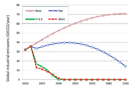
Figure 3 - Global CO2 Emissions from NBER Paper

Figure 4 - Temperature Change from NBER Paper
There is no 1.5 degree or 2.0 degree limit case in the paper and looking at the reduction in carbon dioxide emissions required for a 2.5 degree limit, those targets do indeed look practically impossible. In the base case, Figure 4 shows the world would be more than 4 degrees centigrade warmer in 2100 and in the optimal case, it would be about 3.5 degrees warmer. Referring to Figure 3, there is a very substantial decrease in carbon dioxide emissions required to achieve that relatively small difference in outcome.
Figure 5 shows the cost to society of carbon dioxide emissions under the various scenarios using data from the NBER report. Table 1 shows the cost of carbon dioxide emissions on an annualized basis using data taken from the NBER report. There are two conclusions from Figure 5. The first is that the optimal path imposes the lowest costs on society. The second is that the base case imposes significantly lower costs than trying to limit global warming to 2.5 degrees centigrade in 2100.

Figure 5 - Societal Cost of Climate Change
From Table 1, we can see that there is no real difference in the annual cost of carbon between base and optimum scenarios. The difference between the two is that there is less damage under the optimal case and more abatement. The real benefits of the optimal case are realized in the second half of the century.
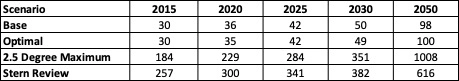
Table 1 - Social Cost of Carbon Annually ($ / Ton)
There are some legitimate criticisms of this approach. After all, none of us live in an economic model, but in a world that will be noticeably warmer. Like all models it is, at best, directionally correct and over long time horizons economics discounts away damage in the distant future. It does, however, provide a tool to estimate the costs and benefits of action, which is a lot better than no tool at all.
What would be the impact of imposing a carbon tax of $50 or $100 per ton on oil demand? Columbia’s Center for Global Energy Policy have looked at the impact for energy demand in the United States based on carbon taxes of between $0 and $73 per ton (viii). Their conclusion was that a tax would result in a substantial reduction in carbon dioxide emissions but would have almost no impact on oil demand. This is because a carbon tax works by eliminating the cheapest emissions first; the Colombia paper found that almost all the reduction in emissions came in the power sector, where renewables and natural gas replaced coal, because those replacement fuels are already economically competitive. A carbon tax of $50 per ton would equate to a $0.44 dollar per gallon tax on gasoline. This is about 20% of the cost of the average 2016 tank of gasoline, which was $2.30, an increase which falls well within the range of fluctuations in gasoline prices driven by the oil price. Table 2 shows the impact on a gallon of gasoline for the carbon taxes shown in Table 1.
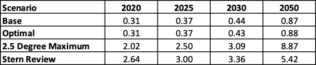
Table 2 - Additional Tax on Gasoline ($/Gallon)
The Colombia study did not examine the impact of the $2 plus taxes on carbon emissions, but it isn’t hard to imagine that doubling, tripling and then quadrupling the cost of gasoline would have a dramatic impact on demand.
Bringing the discussion back to long term oil demand forecasts, this divergence in carbon rates under different scenarios can explain the divergence in forecasts. The ‘above the line’ forecasts, those that predict demand rising for the next decade or two, follow a base or optimized carbon price path, where abatement of carbon dioxide emissions will be focused on the power sector. The ‘below the line’ forecasts follow a temperature limited path, where the abatement impact of the mobility sector are dramatic and immediate.
It seems unlikely that society would be willing to accept, or that politicians could be reelected after imposing, the kinds of costs that would be required to achieve the ‘below the line’ forecasts. It is hard to imagine the US government attempting to impose a $2 per gallon gasoline tax and increasing it at 10 cents per year. The aggressive bp forecasts and the IEA sustainable development case would restrict temperature rise to 1.5 degree or below 2.0 centigrade, implying even higher gasoline taxes than that. The ‘above the line’ forecasts reflect not only the economic optimum, but also the political reality, which means that oil demand can be expected to continue to grow for the next ten to twenty years.
Implications for the E&P Industry
If we adopt this oil demand scenario, what are the implications for the E&P industry? Some media coverage earlier this year suggested that the COVID-19 pandemic foreshadowed what this decline in demand would look like for the industry. As a reminder, if any were needed, April this year saw oil demand collapse by 12.4 MMbbl/day month on month at the same time as Saudi Arabia initiated a price war by adding 2 MMbbl/day to global supply. This doesn’t seem a suitable analogue for structural demand decline, which is likely to be gradual and sustained over decades. It is likely that peak demand won’t be recognized until several years after the event, and post plateau underlying demand decline rates of 1%-2%, of a similar magnitude to pre-plateau demand growth rates, seem more likely.
What are the implications for the industry under this scenario? The major international oil companies have consistently pointed out that the world will need oil, and new supplies of oil, for decades to come, which is consistent with the scenario outlined here. The emphasis has been on developing assets with low breakeven prices, so that when demand declines, those assets will remain competitive while assets with higher break evens will have their production pushed out of the market. This strategy makes intuitive sense. Does that mean that business will continue as normal?
Figure 6, below, is taken from a recent press release by Rystad Energy (ix). This figure shows the breakeven price of oil supply, broken out by theme. Breakeven prices are on a point forward basis and it appears that averages are used rather than actual field data, as the legend indicates a 60% confidence interval around the average breakeven price presented.

Figure 6 - Oil Supply Cost Curve
Figure 6 distinguishes between producing and non-producing fields and the key takeaway from this chart is that, using average costs on a point forward basis, there is no field development theme that can compete with existing production. Figure 6 is a simplification, within each theme there will obviously be a range of breakeven prices, which will change for each field over time as production declines with age. There will also be fields, in the middle east and perhaps deep water fields in places such as Guyana and Brazil, that can compete with existing production, even including their capital cost. Notwithstanding these points, broadly speaking non-producing fields will struggle to compete with producing fields on breakeven price. This conclusion makes intuitive sense, after all, non-producing fields still require capital investment to bring them on stream, whereas for producing fields, that is a sunk cost. This implies that new production from non-producing fields will not displace existing production from producing fields.
The second point of difference between existing production and non-producing fields is how operational and investment decisions are made. In a producing field, the decision on whether to continue or suspend production is made on the basis of whether the field can be operated profitably, together with a consideration of the value of deferring abandonment. Oil price risk can be transferred by hedging production over the next year or 18 months. Decisions are made over a short time horizon with high certainty. Compare this to a non-producing field. Even those fields that are ready to take a Final Investments Decision are years away from realizing first production, with the return on investment then being made over a further 15 to 30 year period. There is no way to transfer price risk by hedging. In contrast to existing production, decisions are taken over very long time horizons with high uncertainty. The investment case has worked historically because oil demand was rising. How can a company justify the risk associated with that kind of long term investment when demand declines?
The implication of this second point is that investment in new oil fields will cease once demand begins to decline. It won’t, of course, stop everywhere at once, but it will taper down with the only the most profitable, short cycle fields continuing to attract investment, until eventually even those are considered to be too high risk.
What does this type of scenario mean for the industry today? In the first instance, the role of exploration in the oil and gas industry will change; it will shrink and shift in focus to infrastructure led opportunities that can be quickly monetized. BP has already announced that it is moving down this route, by abandoning exploration in new basins. Their timing may turn out to be prescient but given the assumption of another decade or two of demand growth, it seems a little early. There are still a lot of high value exploration opportunities available and enough time to monetize them.
This scenario also calls into question the industries current strategy of focusing on fields with low breakeven prices, at least for the next decade or so. Of course, low breakeven prices are always important to the extent that they are also a reflection of overall field profitability, but providing the field is sanctioned within the next decade or two, that production will not be displaced. Under this scenario, low operating costs will be more important over the long run than low lifecycle breakeven prices.
What does the future oil market look like under this kind of scenario? It is intuitive to think that a world in which oil demand declines would be characterized by consistently low prices. But a world in which demand declines at 1%-2% while underlying production declines at 5% and there is no material new investment, is a world in which oil prices would soar. This would be a world in which field redevelopment and infill drilling opportunities could become highly profitable, but they are unlikely to be enough to fill the void.
The kind of asset that would really win in this environment would be one that has no exploration risk, could be brought on stream in months rather than years and which realizes the bulk of its economic value over a time horizon where price risk can be transferred through hedging. If this description sounds familiar, it should. US shale is the ideal asset for a world where oil demand is declining as it has exactly those characteristics. It may turn out that the US shale revolution of the last decade was just a couple of decades early.
To summarize, the scenario presented here is one in which oil demand continues to rise for the next decade or two, plateauing and beginning a slow and steady decline. Once this occurs, investment in new oil and gas fields will quickly decline, resulting in price spikes as underlying field production declines outstrip the decline in supply. US shale becomes the asset of choice, given its short cycle times and the ability to realize most of the value within 18 months of investment.
The best strategy for an oil and gas company to pursue under this scenario is to invest in long life assets with low operating costs, not necessarily the assets with the lowest lifecycle breakeven prices. Maintain an active exploration program, including new basin exploration, and only begin to exit these positions when the projected first oil dates from these fields moves beyond 2035 – 2040. Take advantage of the currently depressed US shale industry to assemble a competitive shale position; a position that can be held over the long term with minimum work commitments. While this is an oil focused article, continuing to invest in profitable gas and renewable opportunities should also form part of this strategy.
(i) IEA (2020), World Energy Outlook 2020, IEA, Paris https://www.iea.org/reports/world-energy-outlook-2020
(ii) “International Energy Outlook 2020”, Energy Information Administration, October 2020
(iii) World Oil Outlook 2045, October 2020, OPEC
(iv) Energy Outlook 2020 Edition, September 2020, bp
(v) Global Energy Perspective: Accelerated Transition, November 2018, Energy Insights by McKinsey
(vi) “Projections and Uncertainties about climate change in an era of minimal climate policies”, National Bureau of Economic Research Working Paper 22933, William D. Nordhaus, September 2017.
(vii) “Climate Change: Our Ultimate Challenge”, William Nordhaus, Lecture at the University of Zurich, January 21st, 2020.
(viii) “Energy and Environmental Implications of a Carbon Tax in the United States”, Columbia Center on Global Energy Policy, July 2018.
(vix) “Oil production costs reach new lows, making deep water one of the cheapest sources of novel supply”, Rystad Energy, October 21st, 2020.
Conversation


Explore Our Services
Business Development
Oil & Gas an extractive industry, participants must continuously find and develop new oil & gas fields as existing fields decline, making business development a continuous process.

Strategy
We approach strategy through a scenario driven assessment of the client’s current portfolio, organizational competencies, and financial framework. The strategy defines portfolio actions and coveted asset attributes.

Origination
Deal origination consists of identifying coveted assets, assets with attributes consistent with the client’s strategy, and qualified buyers. We advocate a proactive approach to business development and will undertake outreach on our client’s behalf.
Transaction Support
Transaction support consists of in depth asset evaluation, negotiation of commercial agreements or preparation of license round submission and close out of conditions. We can also aid in joint venture set up and management and asset maturation as required.